38 excel 2010 chart axis labels
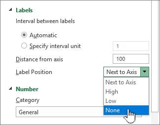
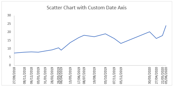
› skip-dates-in-excelSkip Dates in Excel Chart Axis - My Online Training Hub Jan 28, 2015 · Right-click (Excel 2007) or double click (Excel 2010+) the axis to open the Format Axis dialog box > Axis Options > Text Axis: Now your chart skips the missing dates (see below). I’ve also changed the axis layout so you don’t have to turn your head to read them, which is always a nice touch. c# : Excel 2010: Excel.Chart -> X Axis -> Hide the labels This should be an easy to answer question, but I cannot find out how to solve it. I have a Excel.Chart object, which has an Excel.Axis -> an x-axis. I want to hide / switch off the displaying of the labels in the axis (but leave the rest of the x-axis, i.e. not to delete it) . How could this be ... · Excel.XlTickLabelPosition.xlTickLabelPositionNone ...
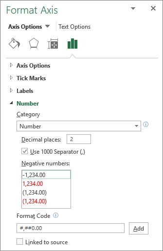
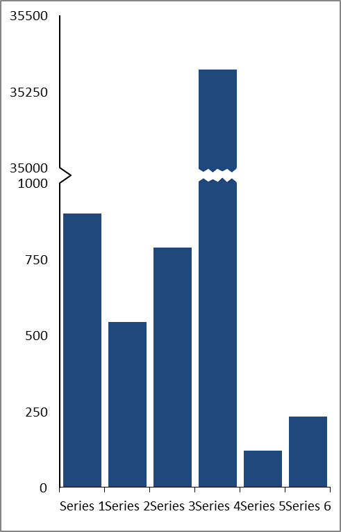
peltiertech.com › broken-y-axis-inBroken Y Axis in an Excel Chart - Peltier Tech Nov 18, 2011 · – For the axis, you could hide the missing label by leaving the corresponding cell blank if it’s a line or bar chart, or by using a custom number format like [<2010]0;[>2010]0;;. You’ve explained the missing data in the text.
Excel 2010 chart axis labels
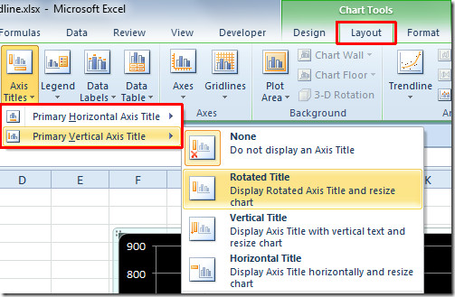
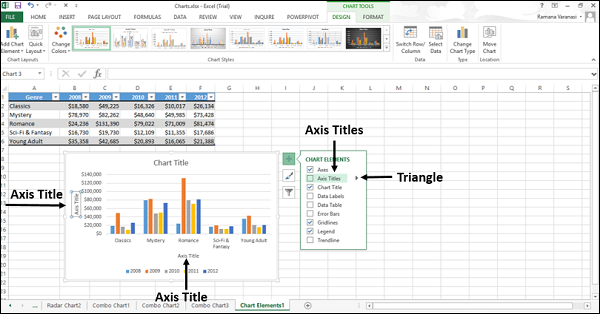
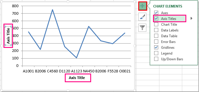
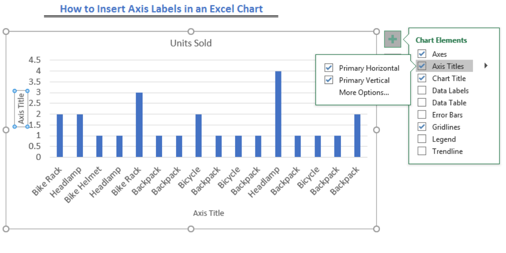
Excel charts: add title, customize chart axis, legend and data labels Click anywhere within your Excel chart, then click the Chart Elements button and check the Axis Titles box. If you want to display the title only for one axis, either horizontal or vertical, click the arrow next to Axis Titles and clear one of the boxes: Click the axis title box on the chart, and type the text. How to add axis label to chart in Excel? - ExtendOffice If you are using Excel 2010/2007, you can insert the axis label into the chart with following steps: 1. Select the chart that you want to add axis label. 2. Navigate to Chart Tools Layout tab, and then click Axis Titles, see screenshot: 3. You can insert the horizontal axis label by clicking Primary ... How to Label Axes in Excel: 6 Steps (with Pictures) - wikiHow Steps Download Article. 1. Open your Excel document. Double-click an Excel document that contains a graph. If you haven't yet created the document, open Excel and click Blank workbook, then create your graph before continuing. 2. Select the graph. Click your graph to select it. 3.
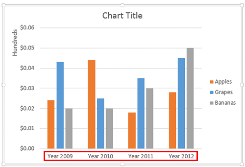
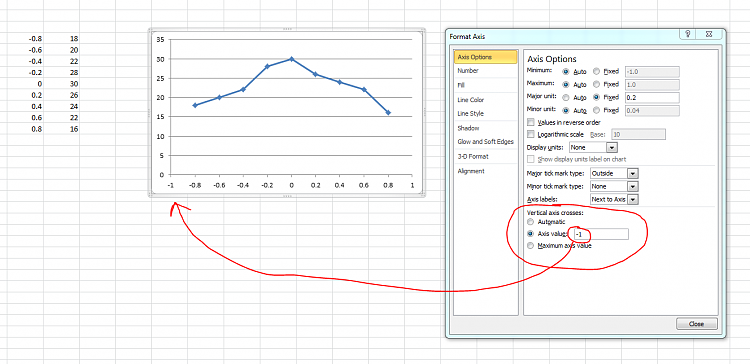
Excel 2010 chart axis labels. How to Add Axis Labels in Excel Charts - Step-by-Step (2022) - Spreadsheeto How to add axis titles 1. Left-click the Excel chart. 2. Click the plus button in the upper right corner of the chart. 3. Click Axis Titles to put a checkmark in the axis title checkbox. This will display axis titles. 4. Click the added axis title text box to write your axis label. vertical grid lines for multi-level category axis labels For the secondary axis label, select only the years (one row) instead of multilevel with year and month (two rows). Go to Layout/Axes and plot the secondary axis on top. Select the secondory axis on top. Then go to the Layout/Gridlines and add a secondary vertical gridline. Then just select the secondary axis on top and delete it. That is it. support.microsoft.com › en-us › officeChange axis labels in a chart - support.microsoft.com Your chart uses text from its source data for these axis labels. Don't confuse the horizontal axis labels—Qtr 1, Qtr 2, Qtr 3, and Qtr 4, as shown below, with the legend labels below them—East Asia Sales 2009 and East Asia Sales 2010. Change the text of the labels. Click each cell in the worksheet that contains the label text you want to ... How to Change Axis Labels in Excel (3 Easy Methods) For changing the label of the vertical axis, follow the steps below: At first, right-click the category label and click Select Data. Then, click Edit from the Legend Entries (Series) icon. Now, the Edit Series pop-up window will appear. Change the Series name to the cell you want. After that, assign the Series value.
Chart.Axes method (Excel) | Microsoft Learn expression. Axes ( Type, AxisGroup) expression A variable that represents a Chart object. Parameters Return value Object Example This example adds an axis label to the category axis on Chart1. VB With Charts ("Chart1").Axes (xlCategory) .HasTitle = True .AxisTitle.Text = "July Sales" End With Custom Axis Labels and Gridlines in an Excel Chart The labels are (temporarily) shaded yellow to distinguish them from the built-in axis labels. Select the horizontal dummy series and add data labels. In Excel 2007-2010, go to the Chart Tools > Layout tab > Data Labels > More Data Label Options. In Excel 2013, click the "+" icon to the top right of the chart, click the right arrow next to ... › make-histogram-excelHow to make a histogram in Excel 2019, 2016, 2013 and 2010 Sep 29, 2022 · For this, you'd need to change the horizontal axis labels by performing these steps: Right-click the category labels in the X axis, and click Select Data… On the right-hand side pane, under Horizontal (Category) Axis Labels, click the Edit button. In the Axis label range box, enter the labels you want to display, separated by commas. charts - how to check the x axis label in vba (Excel 2010) - Stack Overflow This piece of code is trying to change the colour of the chart bars according to the Quarter (four quarters of a year and the same colour for every other quarter) so my x-axis label is by month and I am trying to search for it and then use the Month () function to get the month number.
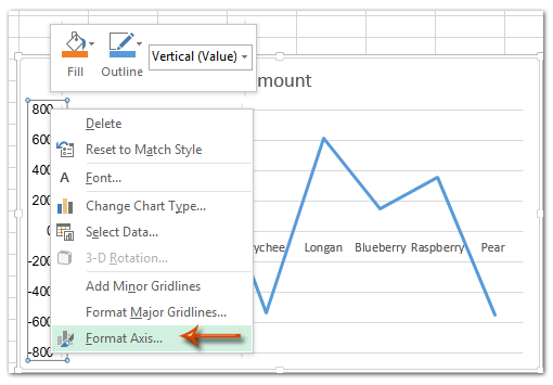
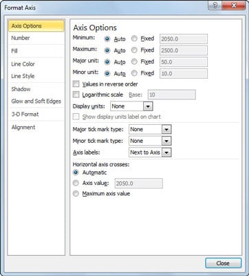
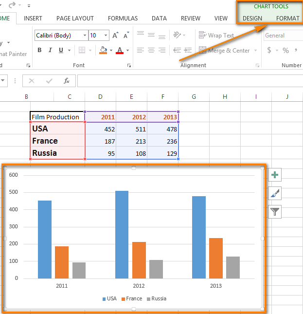
› documents › excelHow to break chart axis in Excel? - ExtendOffice Tip: If you are using Excel 2007 or 2010, right click the primary vertical axis in the chart and select the Format Axis to open the Format Axis dialog box, click Number in left bar, type [>=500]0;;; into the Format Code box and click the Add button, and close the dialog box.) How to group (two-level) axis labels in a chart in Excel? - ExtendOffice The Pivot Chart tool is so powerful that it can help you to create a chart with one kind of labels grouped by another kind of labels in a two-lever axis easily in Excel. You can do as follows: 1. Create a Pivot Chart with selecting the source data, and: (1) In Excel 2007 and 2010, clicking the PivotTable > PivotChart in the Tables group on the Insert Tab; How to Add Data Labels to an Excel 2010 Chart - dummies On the Chart Tools Layout tab, click Data Labels→More Data Label Options. The Format Data Labels dialog box appears. You can use the options on the Label Options, Number, Fill, Border Color, Border Styles, Shadow, Glow and Soft Edges, 3-D Format, and Alignment tabs to customize the appearance and position of the data labels. How to format the chart axis labels in Excel 2010 - YouTube This video shows you how you can format the labels on the x- and y axis in an Excel chart. You can use chart labels to explain what...
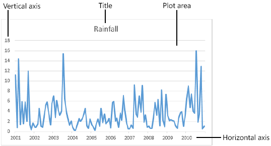
Change the display of chart axes
How to Insert Axis Labels In An Excel Chart | Excelchat We will go to Chart Design and select Add Chart Element Figure 6 - Insert axis labels in Excel In the drop-down menu, we will click on Axis Titles, and subsequently, select Primary vertical Figure 7 - Edit vertical axis labels in Excel Now, we can enter the name we want for the primary vertical axis label.

Format: Chart: Column Chart | Format | Jan's Working with Numbers
Issue with Excel 2010 not displaying all X-axis labels Re: Issue with Excel 2010 not displaying all X-axis labels If you have data with negative values then try moving the axislabel series to the secondary axis. The negative value allow for data labels to be positioned outside end, which forces them down and out of the plot area.
Excel 2010: Insert Chart Axis Title
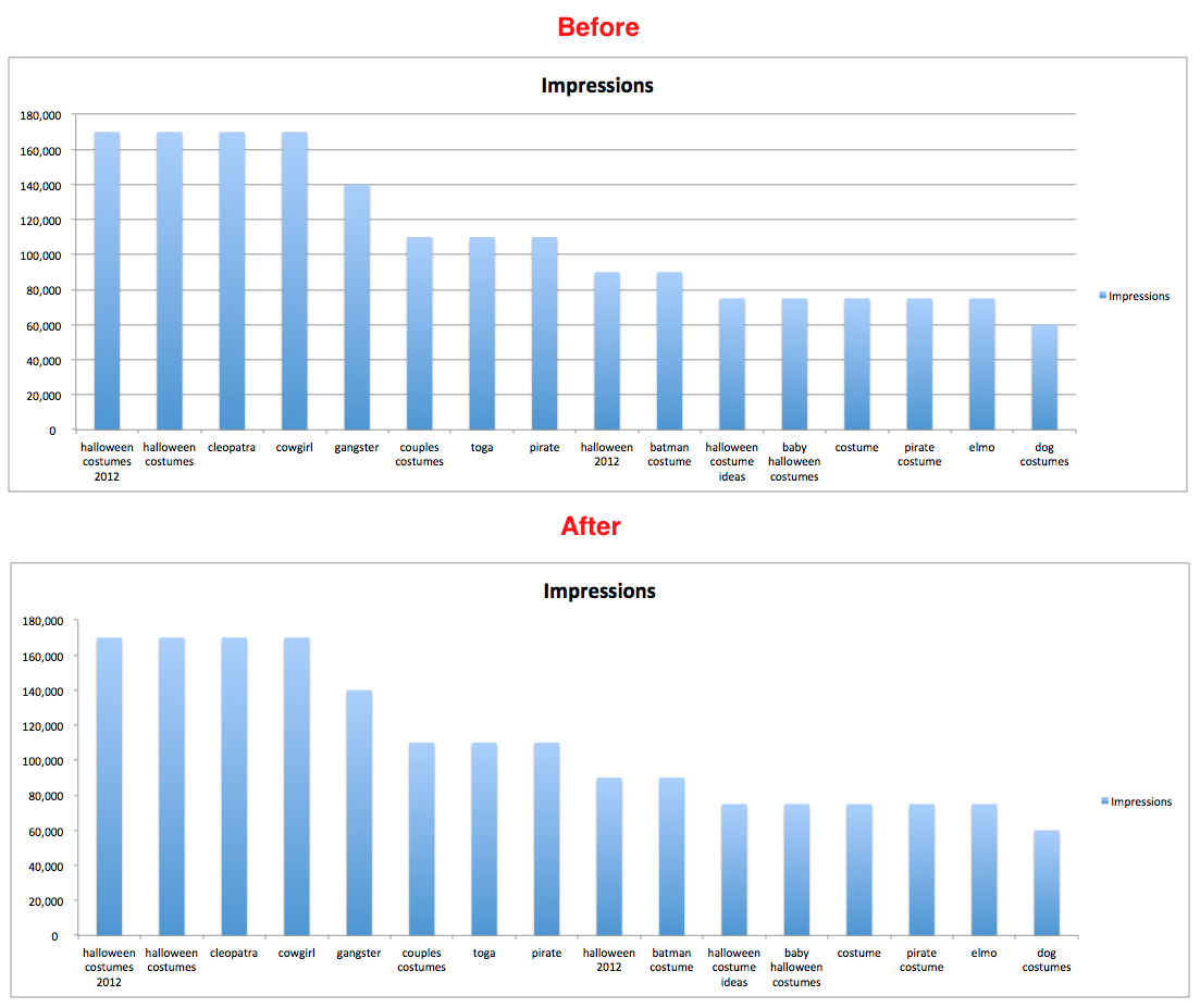
Excel 2010 Problem wrapping x axis labels in a chart 1. Increase the chart area i.e. make its size bigger. 2. Decrease the font size (if you don't want to increase chart size) 3. (Not in your case, but in other cases words some times are big. In these cases, you can make words smaller rather than writing long words) Below is the example where ..... is there and I have increased the chart size.
/Capture-5c7c58fac9e77c0001d19d5b.JPG)
Learn How to Show or Hide Chart Axes in Excel
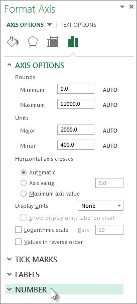
How to Format the X-axis and Y-axis in Excel 2010 Charts Select the axis values you want to format. Click the x-axis or y-axis directly in the chart or click the Chart Elements button (in the Current Selection group of the Format tab) and then click Horizontal (Category) Axis (for the x-axis) or Vertical (Value) Axis (for the y-axis) on its drop-down list.

Add or remove a secondary axis in a chart in Excel
X-axis labels not completely showing in chart - MrExcel Message Board Double-click on the chart along the x-axis. In Format Axis, click on the Scale Tab, and you will see where you can set the maximum value for your x-axis. Enter a value that comfortably covers your x-range. K kcin Board Regular Joined Jun 6, 2006 Messages 118 Jul 30, 2007 #3 Sorry what I mean is that my labels are not showing up completely.
Changing Axis Labels in PowerPoint 2013 for Windows
Excel 2010 charts truncate y-axis labels -- all workarounds found are ... There are hundreds of charts to create on any given production run and having to manually adjust charts is not acceptable, and the truncated labels are not either. Excel 2003 automatically resized the plot area to display the complete text, that is what I need. I have tried every setting possible and cannot find a solution.
Excel Charts - Chart Elements
excel - Dynamic Chart X-Axis labels - Stack Overflow Excel will try to fit all labels on a text X axis, but if it gets too tight, it will omit labels. Format the X axis and select "Specify interval unit" set to 1 if you want to show every label on the X axis. If you leave it at "automatic", Excel may omit labels. Here is the dialog in 2010. Share Improve this answer Follow
How to Change Horizontal Axis Labels in Excel 2010 - Solve ...
superuser.com › questions › 1195816Excel Chart not showing SOME X-axis labels - Super User Apr 05, 2017 · In Excel 2013, select the bar graph or line chart whose axis you're trying to fix. Right click on the chart, select "Format Chart Area..." from the pop up menu. A sidebar will appear on the right side of the screen. On the sidebar, click on "CHART OPTIONS" and select "Horizontal (Category) Axis" from the drop down menu.
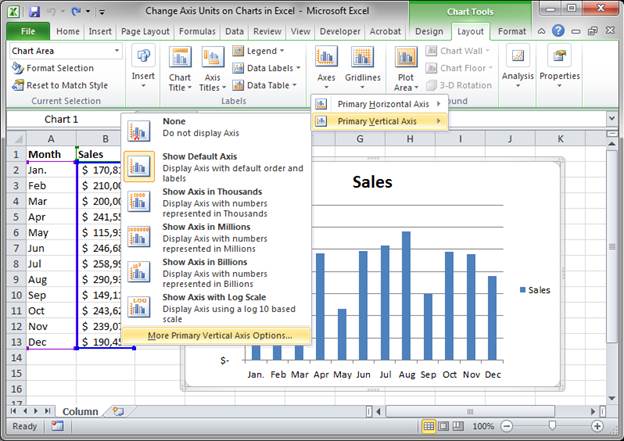
Change Axis Units on Charts in Excel - TeachExcel.com
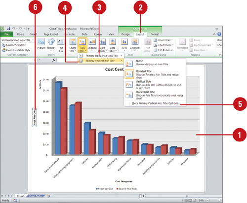
Excel 2010: Insert Chart Axis Title - AddictiveTips To insert Chart Axis title, select the chart and navigate to Chart Tool layout tab, under Labels group, from Axis Title options, select desired Axis Title Position. It will insert Text Box at specified position, now enter the title text. Axis titles can be set at any of available positions.
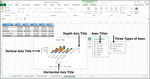
Excel Charts - Chart Elements
How to Add Axis Labels in Microsoft Excel - Appuals.com If you would like to add labels to the axes of a chart in Microsoft Excel 2013 or 2016, you need to: Click anywhere on the chart you want to add axis labels to. Click on the Chart Elements button (represented by a green + sign) next to the upper-right corner of the selected chart. Enable Axis Titles by checking the checkbox located directly ...
Analyzing Data with Tables and Charts in Microsoft Excel 2013 ...
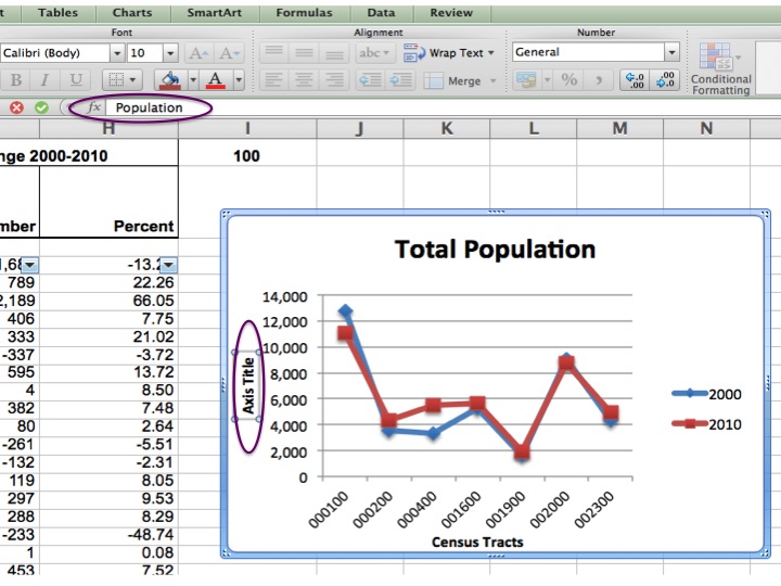
Change axis labels in a chart in Office - support.microsoft.com In charts, axis labels are shown below the horizontal (also known as category) axis, next to the vertical (also known as value) axis, and, in a 3-D chart, next to the depth axis. The chart uses text from your source data for axis labels. To change the label, you can change the text in the source data. If you don't want to change the text of the source data, you can create label text just for the chart you're working on. In addition to changing the text of labels, you can also change their ...
Understanding Date-Based Axis Versus Category-Based Axis in ...
How to add chart titles and axis titles in Excel 2010 - YouTube 2.11K subscribers. This video shows how you can add titles to your charts and to the x- and y-axis of a chart in Excel 2010. 14.
Change axis labels in a chart
Problem with x axis labels in Excel 2010 chart | PC Review Excel Excel 2010 - Chart Axis Text Wrapping Issue: 1: Dec 27, 2012: Remove the weekends from a pivot chart x axis: 0: Nov 5, 2014: Excel conditional formatting of data labels in excel 2003 XY plot: 0: Jul 28, 2009: Excel chart does not start at zero. 1: May 4, 2010: Excel Excel chart and Data Table: 0: Jan 26, 2009

How to Change Excel Chart Data Labels to Custom Values?
How to Use Cell Values for Excel Chart Labels - How-To Geek Select the chart, choose the "Chart Elements" option, click the "Data Labels" arrow, and then "More Options.". Uncheck the "Value" box and check the "Value From Cells" box. Select cells C2:C6 to use for the data label range and then click the "OK" button. The values from these cells are now used for the chart data labels.
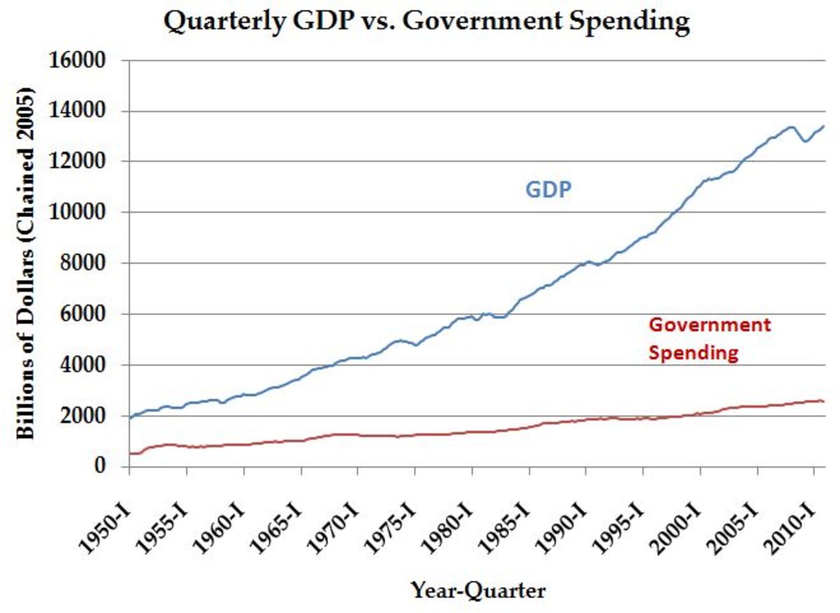
How to Graph and Label Time Series Data in Excel - TurboFuture
chart axis labels are cut off by box - Microsoft Community You could select the horizontal axis and then reduce the size of the font using the buttons on the Home ribbon to make them fit or alternatively you can drag the bottom of the chart area upwards to make more space for the x-axis. I don't know about forcing Excel to make room for rotated labels in future but if you move the chart to its own sheet you should find the labels are displayed ok.
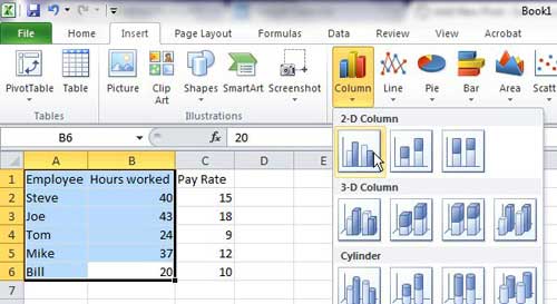
EXCEL Charts: Column, Bar, Pie and Line
support.microsoft.com › en-us › officeAdd or remove a secondary axis in a chart in Excel To complete this procedure, you must have a chart that displays a secondary vertical axis. To add a secondary vertical axis, see Add a secondary vertical axis. Click a chart that displays a secondary vertical axis. This displays the Chart Tools, adding the Design, Layout, and Format tabs.
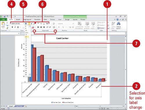
Microsoft Excel 2010 : Formatting Chart Text & Formatting ...
How to Label Axes in Excel: 6 Steps (with Pictures) - wikiHow Steps Download Article. 1. Open your Excel document. Double-click an Excel document that contains a graph. If you haven't yet created the document, open Excel and click Blank workbook, then create your graph before continuing. 2. Select the graph. Click your graph to select it. 3.

How to Label Axes in Excel: 6 Steps (with Pictures) - wikiHow
How to add axis label to chart in Excel? - ExtendOffice If you are using Excel 2010/2007, you can insert the axis label into the chart with following steps: 1. Select the chart that you want to add axis label. 2. Navigate to Chart Tools Layout tab, and then click Axis Titles, see screenshot: 3. You can insert the horizontal axis label by clicking Primary ...
How to change chart axis labels' font color and size in Excel?
Excel charts: add title, customize chart axis, legend and data labels Click anywhere within your Excel chart, then click the Chart Elements button and check the Axis Titles box. If you want to display the title only for one axis, either horizontal or vertical, click the arrow next to Axis Titles and clear one of the boxes: Click the axis title box on the chart, and type the text.
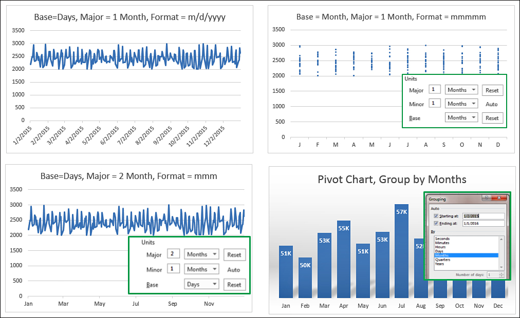
Show Months & Years in Charts without Cluttering » Chandoo ...
Charts | Empirical Reasoning Center Barnard College

Microsoft Excel Tutorials: Format Axis Titles

How to add secondary axis in a chart in Excel 2010? - Insight ...

Manually adjust axis numbering on Excel chart - Super User
Change the display of chart axes
10 Tips To Make Your Excel Charts Sexier

charts - How do I create custom axes in Excel? - Super User
How to add axis label to chart in Excel?
How to Insert Axis Labels In An Excel Chart | Excelchat

Add axis label in excel | WPS Office Academy
secondary horizontal axis – User Friendly

Axis Titles in PowerPoint 2011 for Mac
Solved Excel 2010 Chart Left Axis is in middle of chart ...
Label Specific Excel Chart Axis Dates • My Online Training Hub
Microsoft Excel 2010 - Creating and Modifying Charts ...
How to Format the X-axis and Y-axis in Excel 2010 Charts ...
How to add titles to Excel charts in a minute

Excel Add Axis Label on Mac | WPS Office Academy
Post a Comment for "38 excel 2010 chart axis labels"